Bálint Mazzag and I participated in the QuantChallenge organized by Morgan Stanley, where we competed against 120 teams. Our hard work and determination paid off as we secured the 2nd place at the finals. This post presents our solution to first task.
Codes are available at the corresponding GitHub repository.
Abstract 
We applied several machine learning and ensemble models to predict yields of corn, oats and soybeans. Our approach involved splitting historical data into training and testing sets. We utilized a walk-forward cross-validation method for tuning hyperparameters and testing the performance of the models to avoid overfitting with the aim that they produce reliable out-of-sample performance. LightGBM performed better than other base learners and stacked ensembles. We claim that the use of this model is appropriate to assess the climate risk of the investment, since its performance is stable on testing set and very close to currently published state-of-the-art methods even under the specified conditions.
Introduction
In this paper, we describe our framework to predict yearly crop yields in the counties of Minnesota. Accurately predicting crop yields is critical for farmers, policymakers and investors to make informed decisions related to agriculture. The climate is a crucial factor in crop production, and we aim to build a model based on weather data, including minimum, maximum and average daily temperatures and daily precipitation.
To conduct the analysis and come up with a model, we took into account three main factors during the process: (1) The agricultural specificities (mainly corn grain) of the investigated crops, (2) existing best practices and literature regarding such analysis and forecasting (3) tailoring our approach and model to be generic enough to predict crop yields regardless of geographic information.
Our research on corn yield prediction gave us insights into the modeling approaches that were successful in the past, namely ensemble learning methods that encompass Least Absolute Shrinkage and Selection Operator (LASSO), Random Forest, Support Vector Machine (SVM) and also LightGBM models. Other academic papers applied Long Short-Term Memory (LSTM) models and they were found to be effective in predicting crop yields (Sun et al. 2019). We present a solution to combine the approach of these two existing competent methods first to predict corn yields in Minnesota counties, then for the rest of the crops in question.
Data
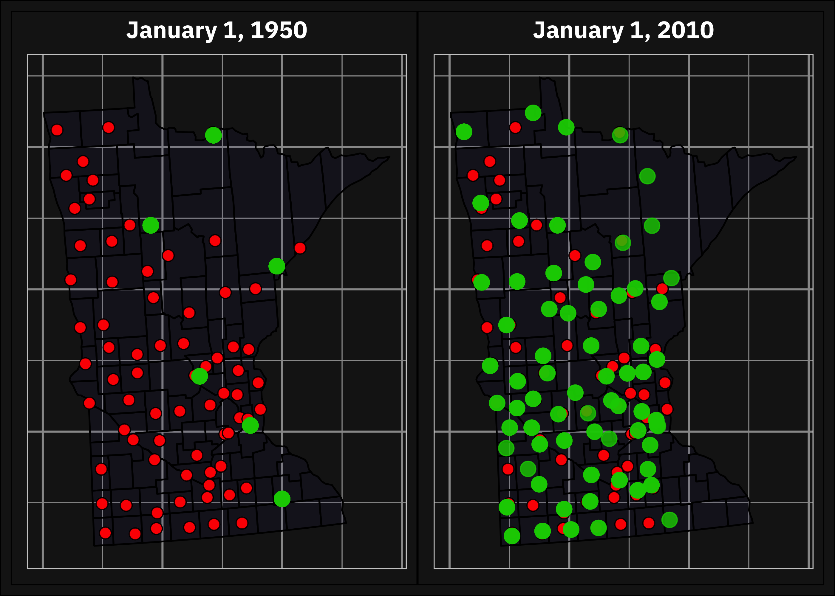
Our selection for the applied methodology was determined by the structure of the data and firstly, we focused our research on corn grain yield prediction. We got the daily data (minimum, maximum, average temperature and perception) of weather stations in Minnesota and annual corn yield statistics of each county in Minnesota from 1950 to 2020. Our goal was to predict the corn yield for a dataset (prediction target) that contains the same weather information for a period from 1991 to 2022, but its geographic location is anonymized.
Before combining the different datasets, we performed data cleaning and preprocessing steps. To handle missing values in the weather data, we applied Multivariate Imputation by Chained Equations (MICE). It is particularly useful, as it enables us to estimate missing data points by considering the relationships between variables. In the case of precipitation, which was frequently missing (63% in the weather dataset used for model building1, 37% in the prediction target set), MICE allowed us to simulate realizations that are most likely given the weather patterns of similar days, what was the weather like on the same day and in the same location at adjacent times. We also applied this strategy on the prediction target set, where we added the observations from weather dataset to give even more accurate data.
This preprocessing step imputed the missing values redundant for the temperature values and ensured that we were working with a complete dataset complete already implies you don’t have missing values. In the case of minimum and maximum temperature, the missing rate was below 1%, and about 9% for the average temperature. Following the literature, we used the average of the minimum and maximum temperature to calculate the average temperature, where it was originally missing. We noticed that the average temperature in the data is very close to the mean of the two limit measurement and this is a reliable approximation method.
After preprocessing the weather data, we merged it with the corn yield statistics by county and year to create a single dataset. In doing this we faced two challenges. The first challenge was to match the geographic locations of weather stations and counties accurately. The latitude and longitude coordinatES of the counties were given in the dataset and also for the weather stations. Even though we imputed the missing values in the database, we still did not have weather data for per day per station for the period under study. The stations were installed at different points in time, so in some cases, there was no observation at all for the given day. To address this issue, we calculated the distance between each weather station (based on Hijmans (2022)) and county to determine which three stations were closest to a given county and we assigned the distance-weighted average values to the counties.
The second challenge we faced was dealing with the differences in temporal granularity between the weather data and yield statistics. The weather data had a daily time granularity while the corn yield statistics were at an annual frequency. One possible solution is to use each day’s observation of the weather data as a predictor and combine the two datasets based on the year and the distance. After some initial attempts, we realized that this leads to a very small observation-to-feature ratio and overfitting in the built models. Shahhosseini, Hu, and Archontoulis (2020) also described this problem in their study and addressed it through a three-stage feature selection. Following their approach, we aggregated the daily weather data to a weekly level.
Based on the literature of agricultural research we also derived Growing Degree Days (GDD) and Killing Degree Days (KDD). KDD is a concept used to measure the accumulated heat units above a specific temperature threshold that can potentially harm or kill a plant and GDD is a measure of heat accumulation used to predict plant growth stages (Butler and Huybers 2013). It is calculated by taking the average daily temperature above a certain base temperature, which is specific to the plant species. For corn, the base temperature is typically around 9°C (41°F). The threshold for KDD is set at 29°C (Yu et al. 2022; Lin et al. 2020). In the case of oats these values are 7°C and 25°C, while for soybean 12°C and 30°C (Porter and Parry 1993).
Corn is an annual plant, meaning it completes its life cycle within one growing season, from planting (spring) to harvesting (usually ends in October). The case of oats and soybean are the same. But weather in the previous year influence the quality of the soil, hence previous years’ precipitation and temperature could also affect yields. Therefore, we discarded all information from the given year’s November and December and combined them with the previous year’s data from winter. Although the model’s forecast can be improved in this way, it involves the issue that for observations in the prediction target set where we do not have information on the previous year’s weather, it is necessary to build a restricted model that only uses data from the current year.
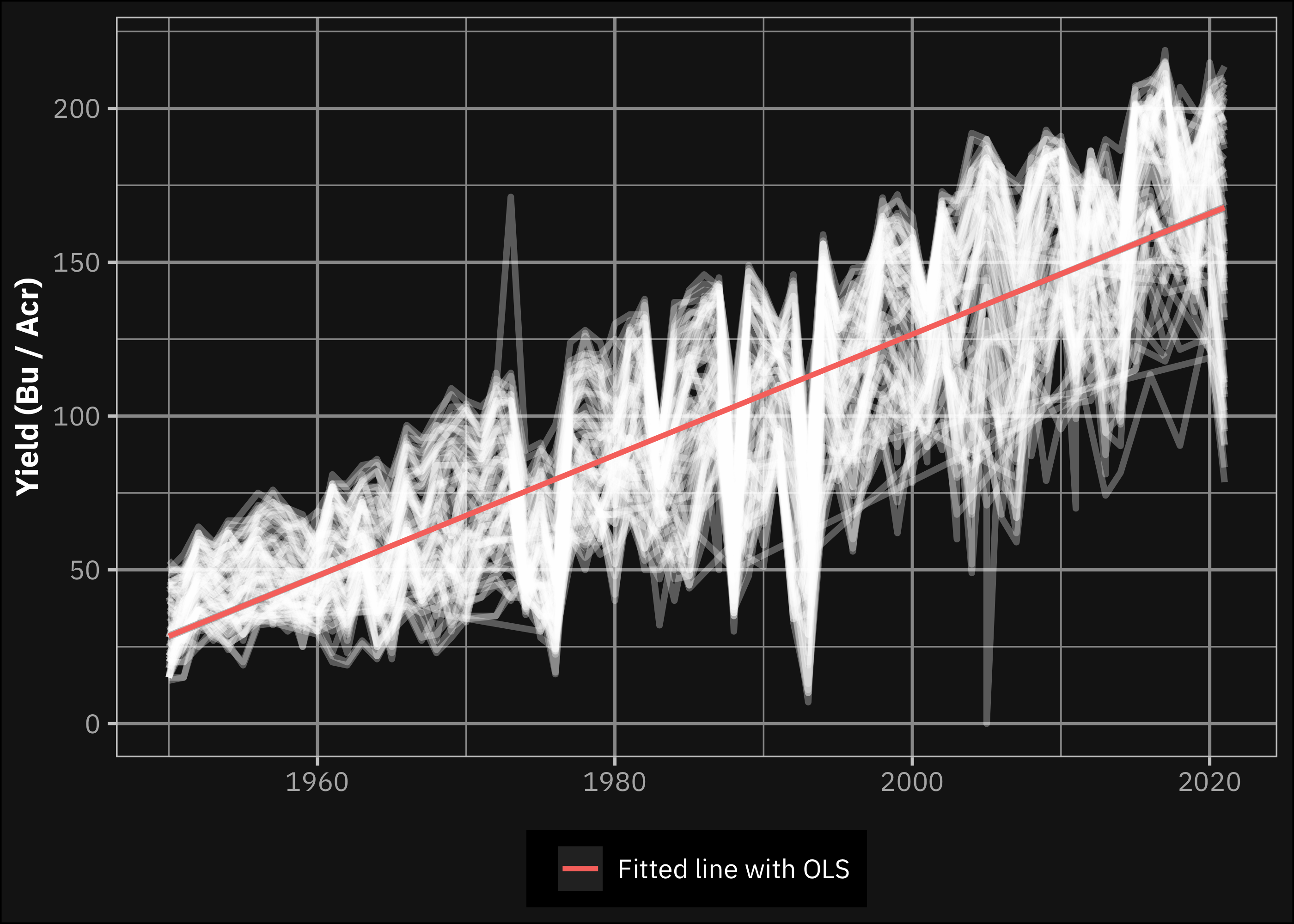
Shahhosseini, Hu, and Archontoulis (2020) presents that an increasing trend in corn yields are observable. This also holds for our data (see Figure 2), but it also shows high fluctuations. Since most of the observations in the prediction target set overlap with the historical dataset we use for modelling, we decided to add year as a predictor to the model instead of subtracting a linear trend of the yields. The existence of this trend means that extrapolation with tree based models may perform low, but the preprocessing step Shahhosseini, Hu, and Archontoulis (2020) used also does not solve this issue. But applying year as a predictor may significantly improve the prediction ability if it is not the case of extrapolation. Since we apply walk-forward cross-validation for training and testing, our models may perform even more accurately, when predicting the yields for the prediction target set.
Methodology
To find an appropriate model that could accurately predict corn yields, we found the collection of existing articles and their reported forecast accuracy in Shahhosseini, Hu, and Archontoulis (2020) to be a good starting point. They highlight that their ensemble model outperformed other models in predicting corn yields when they used walk-forward cross-validation for evaluation (RMSE = 1,138 kg/ha). There exist in the literature other approaches, but the majority of these are not fit to our goal. Some methods produced better predictions with the application of other weather and soil-related variables, such as MODIS sensors or irrigation, but in our current case, the weather data was given. Jeong et al. (2016) reported smaller RMSE values with random forest, but their validation method was not walk-forward cross-validation, which we found to be crucial in accurately evaluating our model, otherwise, the performance of the model may be questioned for a period outside the sample (extrapolation).
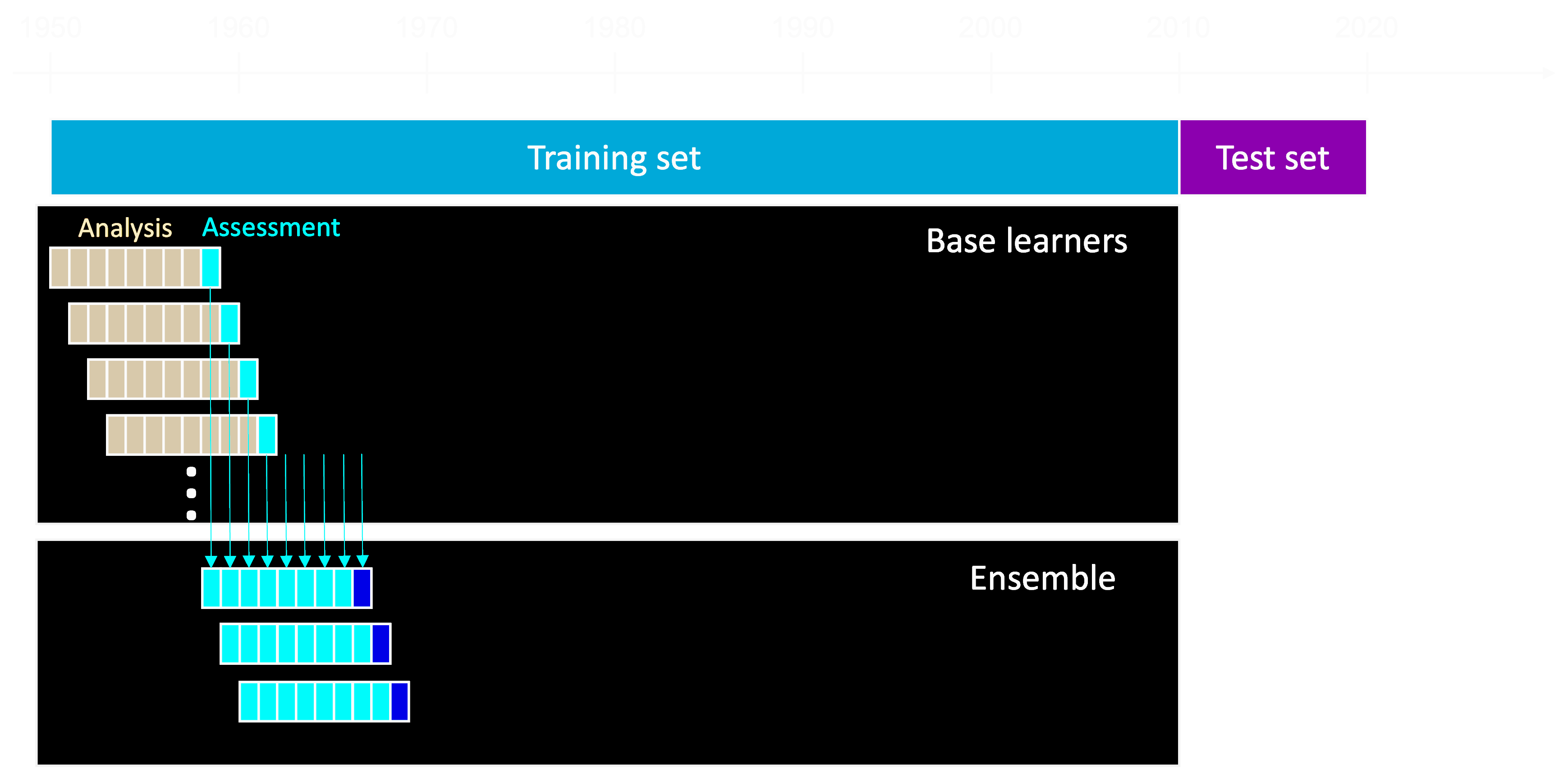
Shahhosseini, Hu, and Archontoulis (2020) states that combining multiple machine learning models could lead to better forecasting results than a single model if the base learners are diverse. To this end, we used a stacked ensemble of five2 diverse models (base learners): LASSO, linear SVM, lightGBM, multivariate adaptive regression splines MARS and random forest. We splitted our historical data initially into training (before 2010) and testing sets (after 2010). Subsequently, we applied a walk-forward cross-validation method in which the 8-year analysis and 1-year assessment sets were shifted one year at a time.
We tuned the hyperparameters of the applied base learners using grid search to minimize the resulted root mean squared error (RMSE) on the assessment sets, while they were trained on the analysis sets. We selected RMSE as the target metric, to produce comparable results with the existing literature.
We applied three models to build the stacked ensemble models based on the prediction of the base learners: ordinary least squares (OLS), LASSO and (MARS). To tune the hyperparameters of these models we generated predictions from the previously mentioned diverse base learners for the assessment sets and we used the previously mentioned walk-forward cross-validation. These sets contain substantially fewer variables (only the predictions from the four base learners) and the number of sets is also lower since we drop the first eight years. But this does not influence our final selection, because we compare the performance of the models on the test set which is held out and unseen during the training process.
This method allows us to identify the best-performing stacked ensemble model (or a base learner) based on its performance in predicting corn yield with the possibility of extrapolation.
We also extended our methodology with a geometric weighting of the observations based on the year. This approach is also known as Koyck lag (Koyck 1954), and it aimed to give more emphasis to the more recent observations, as they are expected to be more relevant for predicting the current corn yield. The theoretical justification for this approach is that several technological improvement in agriculture has been made in recent years, which might lead to changes in the relationship between the climate and corn production.
This weighting was incorporated into our framework by applying importance weights. This means that weights are applied during the model building on the analysis set, but in contrast with frequency weights, these weights do not affect directly the performance indicators related. We extended the original formula with an additional fraction to avoid the bias caused by the unequal number of observations in the different years. The equation above shows how we formed these weights:
\[ weight_{t} = \gamma^{max(T)- t} \frac{min(n)}{n_t}, \]
where \(t\) denotes the current year, \(T\) the set of the year, \(n\) the number of observations per years, and \(n_t\) the number of observation in the current year.
A limitation of this weighting technique is that according to our knowledge, currently there is no implementation of adding weights to SVM and lightGBM models (Kuhn and Wickham 2020). Similarly, in the MARS model there is an implementation for weighting, but it considerably increases the running time and in our case we had to abandon weighting here as well (Hastie and wrapper 2023). In these three cases, we fitted unweighted models.
The mentioned models require additional data preprocessing steps beyond those included in the data section. Most of the models needed normalization of the input variables, scaling them to have zero means and unit variances. Furthermore, we also performed feature selection by removing variables that are highly correlated with other variables. We set this limit to 0.9, to have comparable results with Shahhosseini, Hu, and Archontoulis (2020), who have used the same cutoff.
We consider that doing these preprocessing step on the whole historical dataset at once lead to look-ahead bias as evaluating the predictive ability of the model with an observation in the future based on past information is not a realistic scenario and lead to unreliable performance metrics. Therefore, we evaluated these steps on each analysis step separately.
Results
To present the results of our framework, we start with the base learner models. As we described in the methods section, we used different machine learning algorithms to predict corn yield based on climate data, and we tuned the hyperparameters on the splits generated from the training set. Grid based tuning means that for each model we generated a grid of hyperparameter values and trained the model with each combination, selecting the one that performs best on the assessment sets. We applied the maximum entropy design for tuning, which means that the possible hyperparameter combinations are selected to cover the candidate space well and drastically increase the chances of finding good results (Kuhn and Silge 2022). Figure 4 shows the method for the case of SVM, in the case of this model we tried 900 different set of hyperparameters3.
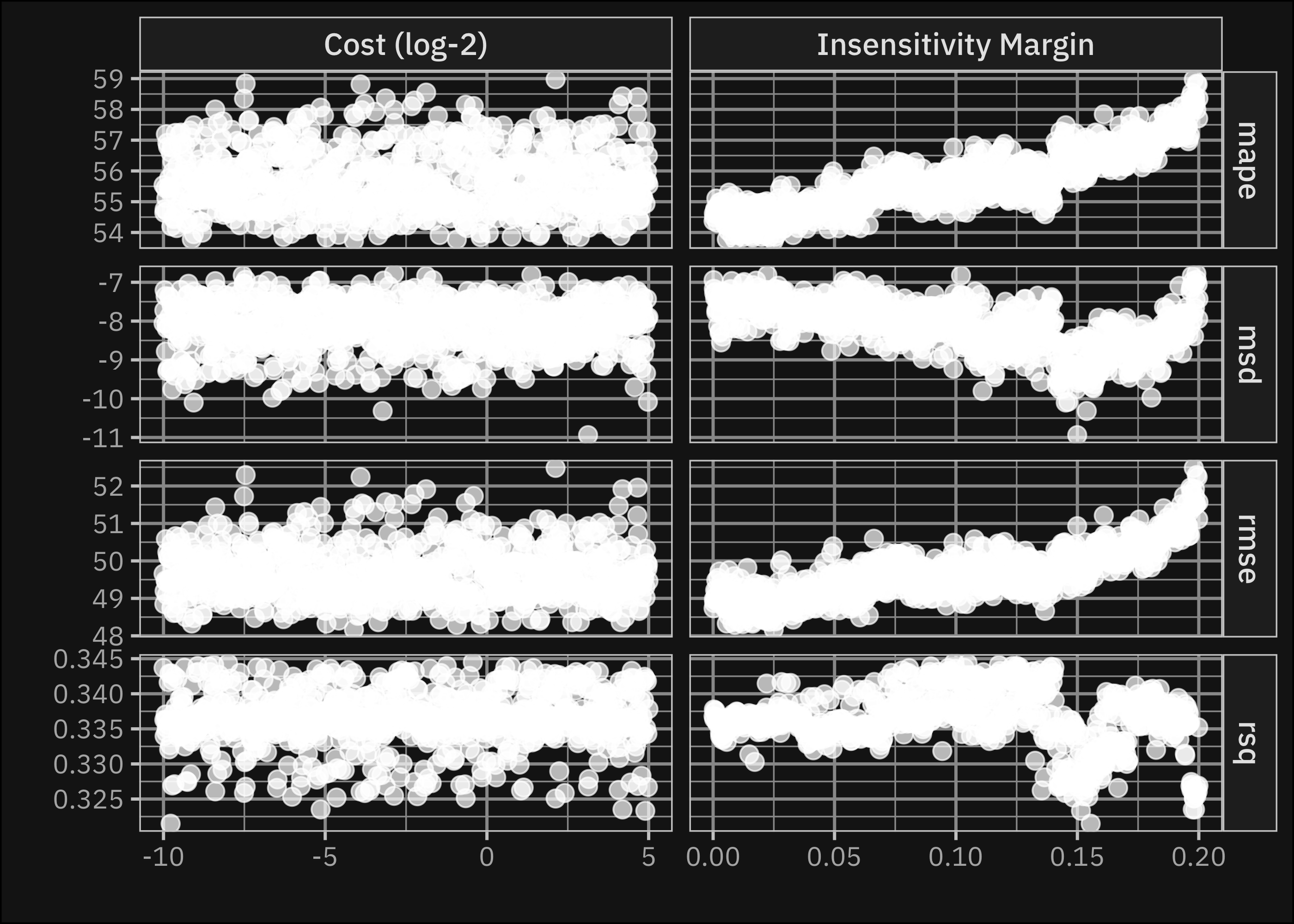
As shown in the figure the optimal values for the hyperparameters are varying based on the targeted performance metric. We decided to minimize the RMSE metric to get comparable results with the literature. The tuned base learner model workflows are reported in the Appendix. Table 1 shows the resulted RMSE values of the tuned models on the testing set (also generated with walk-forward cross-validation).
Table 1: Average RMSE values of the tuned base learner models on the testing set. Values between the parentheses show the standard error (we have 11 assessment sets from the testing data). The \(\gamma\) in the column names refer to the weighting parameter. \(\gamma=1\) means no weigthing used there.
| Engine | \(\gamma\)=0.75 | \(\gamma\)=0.9 | \(\gamma\)=0.95 | \(\gamma\)=1 |
|---|---|---|---|---|
| LASSO | 27.51 (8.83) | 29.17 (9.97) | 29.59 (10.5) | 30.08 (11.4) |
| OLS | 95.90 (67.3) | 80.73 (70.1) | 79.73 (70.2) | 80.55 (71.2) |
| Random forest | 26.47 (6.24) | 25.99 (6.51) | 26.02 (6.45) | 25.60 (6.53) |
| Linear SVM | - | - | - | 47.41 (38.5) |
| MARS | - | - | - | 47.79 (18.9) |
| LightGBM | - | - | - | 24.84 (7.64) |
The results show that the provided weighting method could improve the performance of the LASSO regression. The performance of linear SVM and MARS is significantly lower than the other ML models (we added OLS only as a baseline example). The latter is not surprising, since MARS is especially useful to identify non-linear relationships and interaction effects in the data, but it is suggested to use lower dimensional inputs (Friedman 1991). Hence, we considered an ensemble containing all base learners and another using only the highest-performing models, Random Forest, LASSO and LightGBM. Table 2 shows the performance of the tuned ensemble models on the testing set (parameters of the tuned workflows are reported in the Appendix).
Table 2: Average RMSE values of the tuned ensembe models on the testing set. Values between the parentheses show the standard error (we have 11 assessment sets from the testing data). Values in the Include column refer to the RMSE values, when the ensemble contain all base learners, and values Exclude refer to RMSE, when only the highest-performing models.
| Engine | Exclude | Include |
|---|---|---|
| MARS | 27.32 (6.17) | 30.27 (7.61) |
| LASSO | 26.03 (6.13) | 25.49 (6.5) |
| OLS | 28.50 (6.34) | 30.69 (7.93) |
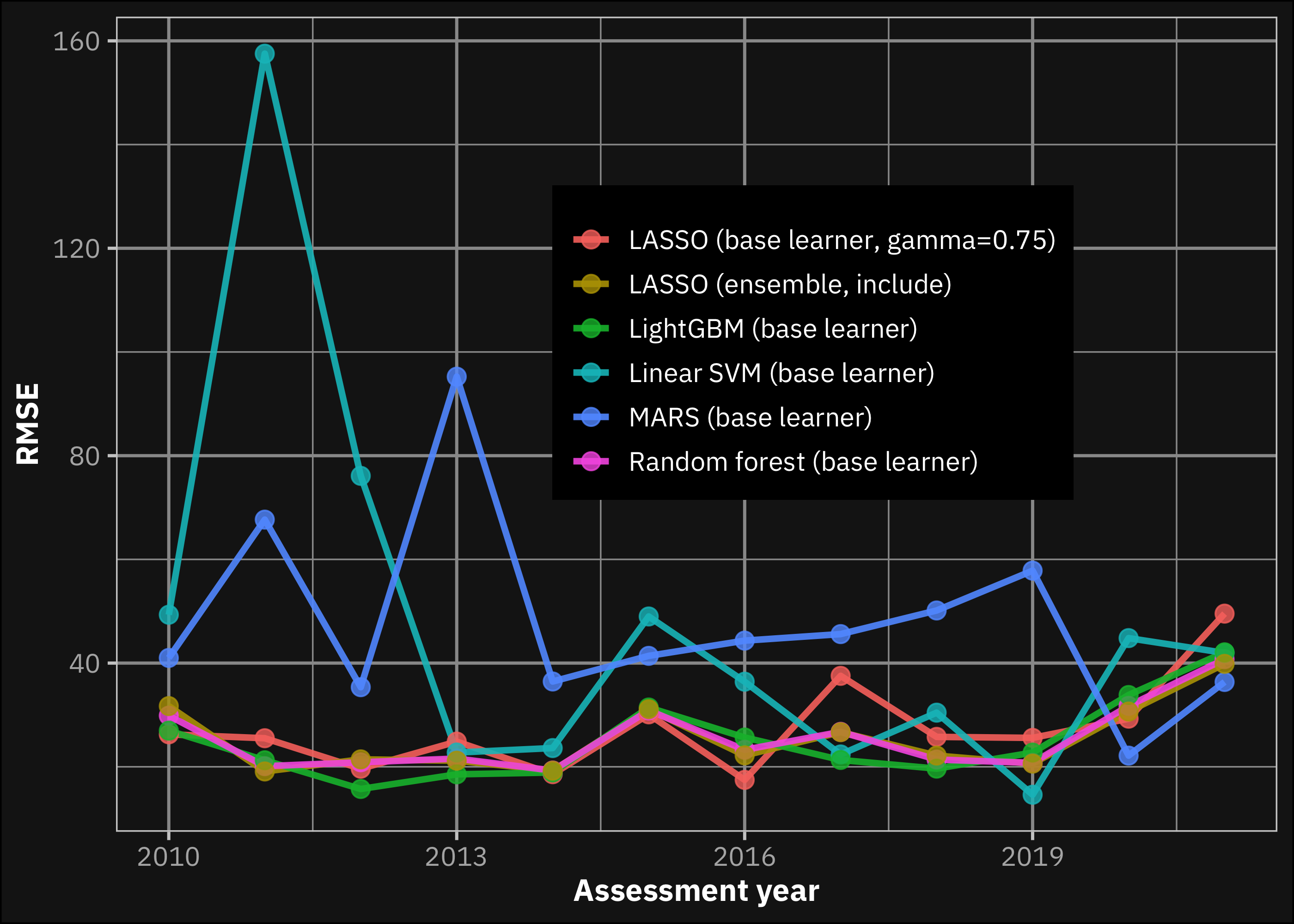
Based on Table 1 and Table 2 we conclude that the best performing model was the LightGBM. The LASSO-based ensemble gave a very close result, with a smaller standard error, that might be advantageous when using for extrapolation (more likely to result the same performance). Figure 5 shows the trend of the performance of the applied models (selected). Based on the figure we do not see, that the performance of any model would considerably outperform the LightGBM in the most recent years. We would highlight this result, because the aim of the analysis is to build a model to assess the climate risk of a bank’s investments in this field, thus the performance in the recent years might be more important than the average performance. But we see that LightGBM is the best performing model based on both evaluation system. Furthermore, the principle of parsimony and the lower computation time are arguments in favor of LightGBM.
In contrast with the results of Shahhosseini, Hu, and Archontoulis (2020), the fact that one of the base learners outperformed the best ensemble model might be possible for the following reasons: (1) We omitted xgboost from the analysis, because of computational bugs that we mentioned earlier. Also important to note that xgboost is ineffective if the prediction requires extrapolation (Bandara, Bergmeir, and Smyl 2020), thus we believe an ensemble with the addition of this model, would not be a clearly better solution. (2) Another reason might be because Shahhosseini, Hu, and Archontoulis (2020) used county level fixed dummy variables, that we could not, because the prediction target is anonymized. This might be the reason also for the higher lowest RMSE that we reached during the analysis (LightGBM results 24.84 bushels/acre, while their best is 1,138 kg/ha, which equals to 18.13 bushels/acre). The relatively lower performance might also be a result of applying walk-forward cross-validation also in the testing process, and they applied another weighting method for ensembling.
Based on the above results, we apply LightGBM to estimate the yields for oats and soybeans. The tuned LightGBM model for these commodities is reported in the Appendix. For these yields LightGBM was even more effective. The average RMSE of the LightGBM predictions for oats was 17.7 bushels/acre and 9.29 bushels/acre for soybeans (evaluated on the testing set).
One limitation of the model is worth mentioning, which can also be seen in the file containing the submitted predictions. LightGBM is tree based model, thus it is expected to perform weakly if the prediction requires extrapolation. If the data is non-stationary then it is possible that predictions remain constant all of them get to the same node. As mentioned earlier observation in the prediction target sets mostly overlap with provided historical dataset. In these cases LightGBM gives accurate predictions. Hence, we trained the final model on the observation after 2006 from the historical dataset and gave predictions based on that. But for the rarely observable old datapoints in the prediction target set, we would suggest using the ensemble or the lasso model instead (we managed these points as they are not the main target in this exercise). We would also suggest the ensemble if our target is assess the climate risk of the investment on the long-run (distribution of the climate might substantially differ).
Conclusion
We have presented a framework for predicting corn yields using machine learning algorithms and ensemble based on climate data. The demonstrated Koyck-lag based weighting could improve the performance of the base learners, but the ensemble still underperformed the LightGBM in terms of RMSE. We applied walk-forward cross-validation to ensure that our model is not overfitted and it produces reliable out-of-sample performance, so it can be used to assess the climate risk of the investment. LightGBM came up with promising results, since its performance on the testing set was consistently better than that of the other algorithms, even in the most recent years. Its performance still falls short compared to the current state-of-the-art methods, but one explanation could be our constraint not to use counties as variables in our prediction, therefore we could not include fixed effect dummies in the model.
Appendix
Tuned base learners
══ Workflow ════════════════════════════════════════════════════════════════════
Preprocessor: Recipe
Model: linear_reg()

── Preprocessor ────────────────────────────────────────────────────────────────
4 Recipe Steps

• step_rm()
• step_zv()
• step_corr()
• step_normalize()

── Model ───────────────────────────────────────────────────────────────────────
Linear Regression Model Specification (regression)

Computational engine: lm

══ Workflow ════════════════════════════════════════════════════════════════════
Preprocessor: Recipe
Model: rand_forest()

── Preprocessor ────────────────────────────────────────────────────────────────
4 Recipe Steps

• step_rm()
• step_zv()
• step_corr()
• step_normalize()

── Model ───────────────────────────────────────────────────────────────────────
Random Forest Model Specification (regression)

Main Arguments:
  mtry = 45
  min_n = 17

Computational engine: ranger

══ Workflow ════════════════════════════════════════════════════════════════════
Preprocessor: Recipe
Model: svm_linear()

── Preprocessor ────────────────────────────────────────────────────────────────
4 Recipe Steps

• step_rm()
• step_zv()
• step_corr()
• step_normalize()

── Model ───────────────────────────────────────────────────────────────────────
Linear Support Vector Machine Model Specification (regression)

Main Arguments:
  cost = 6.54552673129715
  margin = 0.0207393052951536

Computational engine: LiblineaR

══ Workflow ════════════════════════════════════════════════════════════════════
Preprocessor: Recipe
Model: boost_tree()

── Preprocessor ────────────────────────────────────────────────────────────────
4 Recipe Steps

• step_rm()
• step_zv()
• step_corr()
• step_normalize()

── Model ───────────────────────────────────────────────────────────────────────
Boosted Tree Model Specification (regression)

Main Arguments:
  trees = 305
  min_n = 38
  tree_depth = 1
  learn_rate = 0.050851280760922
  loss_reduction = 0.276579958596952
  sample_size = 0.283269332054071
  stop_iter = 13

Computational engine: lightgbm

══ Workflow ════════════════════════════════════════════════════════════════════
Preprocessor: Recipe
Model: linear_reg()

── Preprocessor ────────────────────────────────────────────────────────────────
4 Recipe Steps

• step_rm()
• step_zv()
• step_corr()
• step_normalize()

── Case Weights ────────────────────────────────────────────────────────────────
case_wts

── Model ───────────────────────────────────────────────────────────────────────
Linear Regression Model Specification (regression)

Main Arguments:
  penalty = 0.996509087448771
  mixture = 1

Computational engine: glmnet

══ Workflow ════════════════════════════════════════════════════════════════════
Preprocessor: Recipe
Model: mars()

── Preprocessor ────────────────────────────────────────────────────────────────
4 Recipe Steps

• step_rm()
• step_zv()
• step_corr()
• step_normalize()

── Model ───────────────────────────────────────────────────────────────────────
MARS Model Specification (regression)

Main Arguments:
  prod_degree = 1

Computational engine: earth
Tuned ensembles using all the base learners
══ Workflow ════════════════════════════════════════════════════════════════════
Preprocessor: Recipe
Model: linear_reg()

── Preprocessor ────────────────────────────────────────────────────────────────
2 Recipe Steps

• step_normalize()
• step_zv()

── Model ───────────────────────────────────────────────────────────────────────
Linear Regression Model Specification (regression)

Main Arguments:
  penalty = 0.785607671096585
  mixture = 1

Computational engine: glmnet

══ Workflow ════════════════════════════════════════════════════════════════════
Preprocessor: Recipe
Model: linear_reg()

── Preprocessor ────────────────────────────────────────────────────────────────
2 Recipe Steps

• step_normalize()
• step_zv()

── Model ───────────────────────────────────────────────────────────────────────
Linear Regression Model Specification (regression)

Computational engine: lm

══ Workflow ════════════════════════════════════════════════════════════════════
Preprocessor: Recipe
Model: mars()

── Preprocessor ────────────────────────────────────────────────────────────────
2 Recipe Steps

• step_normalize()
• step_zv()

── Model ───────────────────────────────────────────────────────────────────────
MARS Model Specification (regression)

Main Arguments:
  prod_degree = 1

Computational engine: earth
Tuned ensembles using only high-performing base learners
══ Workflow ════════════════════════════════════════════════════════════════════
Preprocessor: Recipe
Model: linear_reg()

── Preprocessor ────────────────────────────────────────────────────────────────
2 Recipe Steps

• step_normalize()
• step_zv()

── Model ───────────────────────────────────────────────────────────────────────
Linear Regression Model Specification (regression)

Main Arguments:
  penalty = 0.596098767898989
  mixture = 1

Computational engine: glmnet

══ Workflow ════════════════════════════════════════════════════════════════════
Preprocessor: Recipe
Model: linear_reg()

── Preprocessor ────────────────────────────────────────────────────────────────
2 Recipe Steps

• step_normalize()
• step_zv()

── Model ───────────────────────────────────────────────────────────────────────
Linear Regression Model Specification (regression)

Computational engine: lm

══ Workflow ════════════════════════════════════════════════════════════════════
Preprocessor: Recipe
Model: mars()

── Preprocessor ────────────────────────────────────────────────────────────────
2 Recipe Steps

• step_normalize()
• step_zv()

── Model ───────────────────────────────────────────────────────────────────────
MARS Model Specification (regression)

Main Arguments:
  prod_degree = 1

Computational engine: earth
Tuned LightGBM for oats
══ Workflow ════════════════════════════════════════════════════════════════════
Preprocessor: Recipe
Model: boost_tree()

── Preprocessor ────────────────────────────────────────────────────────────────
4 Recipe Steps

• step_rm()
• step_zv()
• step_corr()
• step_normalize()

── Model ───────────────────────────────────────────────────────────────────────
Boosted Tree Model Specification (regression)

Main Arguments:
  trees = 1902
  min_n = 24
  tree_depth = 7
  learn_rate = 4.05162706037683e-10
  loss_reduction = 0.000344450632697509
  sample_size = 0.214169466402382
  stop_iter = 7

Computational engine: lightgbm
Tuned LightGBM for soybeans
══ Workflow ════════════════════════════════════════════════════════════════════
Preprocessor: Recipe
Model: boost_tree()

── Preprocessor ────────────────────────────────────────────────────────────────
4 Recipe Steps

• step_rm()
• step_zv()
• step_corr()
• step_normalize()

── Model ───────────────────────────────────────────────────────────────────────
Boosted Tree Model Specification (regression)

Main Arguments:
  trees = 1792
  min_n = 5
  tree_depth = 13
  learn_rate = 0.0666210324583905
  loss_reduction = 6.36062768974398e-05
  sample_size = 0.469276522332802
  stop_iter = 19

Computational engine: lightgbm
Reference
Footnotes
Considering only the years included in the analysis.↩︎
We ran into a number of technical issues using xgboost, which ultimately led us to abandon its use. As the model created its prediction for the analysis set, a reported computational bug occured that we could solve only with manipulation of the data. Even if this change may not affect the final prediction, it could introduce bias and compromise the model’s accuracy. Another issue was related to its low performance in extrapolating when a value in the assessment set is out of the range of the analysis set. To address these issues, we decided to exclude xgboost from our model stack and continued with the remaining five models.↩︎
Computed in parallel with 9 cores of M1 Pro CPU.↩︎